Utilizing Shuffle Attention for Subject-Wise Split for EEG-Based Alzheimer’s Detection

Introduction

Alzheimer’s disease (AD) is a progressive neurodegenerative disorder characterized by cognitive decline and substantial functional impairment, representing a major public health challenge worldwide [1]. Current diagnostic approaches rely primarily on clinical assessment supported by neuroimaging and cerebrospinal fluid biomarkers, which can be costly, invasive, or limited in accessibility [2]. These constraints have motivated growing interest in alternative modalities that are noninvasive, scalable, and suitable for repeated measurements.

Electroencephalography (EEG) offers a low-cost and noninvasive means of capturing neural activity with high temporal resolution and has been widely studied as a potential biomarker for neurodegenerative disease [3]. Prior work has reported alterations in EEG spectral power, functional connectivity, and signal complexity in patients with AD relative to healthy controls [3], [4]. Building on these observations, machine learning and deep learning techniques have been increasingly applied to EEG data to support automated dementia classification [5]. Many recent approaches employ time-frequency representations, such as short-time Fourier transform or wavelet-based spectrograms, in combination with convolutional neural networks to learn discriminative spectro-temporal features [6], [7].

Despite promising results, a growing body of methodological literature has highlighted limitations in the evaluation protocols used in EEG-based deep learning studies for Alzheimer’s disease. In particular, epoch-wise or slice-wise data splitting can introduce subject-level data leakage because EEG segments from the same individual are strongly correlated. Models evaluated under such conditions may learn subject-specific signatures rather than disease-related patterns, leading to inflated performance estimates that do not generalize to unseen patients. Subject-wise validation strategies, including leave-one-subject-out and patient-level holdout splits, have therefore been recommended to obtain clinically realistic assessments of model performance [8].

In parallel, attention mechanisms have been incorporated into deep learning architectures to enhance feature discrimination by selectively emphasizing informative components of learned representations [9]. Channel-based and spatial attention modules have demonstrated performance gains in a variety of computer vision and biomedical signal processing tasks [10]. However, the application of attention mechanisms to EEG-based dementia classification remains limited, and many existing studies combine attention with validation strategies that do not adequately control for subject-level leakage.

In this study, we investigate a convolutional neural network augmented with a shuffle attention mechanism for binary classification of Alzheimer’s disease versus healthy controls using EEG data. Time-frequency representations derived from short-time Fourier transform spectrograms are used as model inputs, and all evaluations are conducted under strictly enforced subject-wise validation protocols, including both holdout and leave-one-subject-out schemes. By combining attention-based feature refinement with rigorous validation, this work aims to provide a methodologically sound assessment of deep learning performance for EEG-based Alzheimer’s disease classification. The development and execution of this workflow and pipeline were made possible by an open-source pedagogical framework designed to foster collaboration among engineers and researchers alike.

This research was conducted by researchers within Decoded Brain, an active student-led research organization of scientists and engineers focused on collaborative advancement of the brain. Inspired by the traditional peer-review system, engineers at Decoded Brain created a similar structure within the organization to best facilitate research projects and the peer-review process called Open Labs. This open-source software implements a continuous feedback pedagogy where student researchers submit structured weekly progress reports. The literature undergoes a weekly rigorous peer-evaluation process, producing review feedback from fellow research peers that includes technical guidance, directional adjustments, and overall research synthesis. Utilizing this ecosystem allowed the researchers to maintain and foster collaboration and objective peer validation throughout the lifecycle of this paper.

Beyond this specific study, this model is designed for scalability across diverse academic organizations and campuses, with the ultimate goal of fostering decentralized, active research communities. Because the foundational design of Open Labs is inherently domain-agnostic, it can be seamlessly adapted to any field of study. By implementing this framework within institutions—particularly community colleges—we aim to transform the research experience into an enjoyable, deeply engaging, and accessible pursuit, reinforcing that impactful and meaningful technical education is fundamentally a collaborative journey.

Methods

Figure 1 outlines the four principal stages of the proposed pipeline: EEG preprocessing and artifact removal, feature extraction, and classification using the proposed model. Each step will be discussed in detail below to ensure reproducibility and validity.

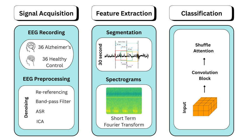
About the EEG

This study used recordings from the 2nd Department of Neurology at AHEPA General University Hospital in Thessaloniki, which are publicly available here. The dataset comprised 36 patients diagnosed with Alzheimer’s disease (AD), 23 patients with frontotemporal dementia (FTD), and 29 healthy controls (HC). Cognitive status was assessed using the Mini-Mental State Examination (MMSE), with scores ranging from 0 to 30 and lower scores indicating greater cognitive impairment. Recordings were acquired and measured from routine EEG of patients in months, and the median value was 25, with the interquartile range (IQR) being 24-28.5 months. Concerning the AD group, no dementia-related comorbidities have been reported. Initial diagnosis of AD and FTD patients was performed according to the criteria provided by the Diagnostic and Statistical Manual of Mental Disorders, 3rd ed., revised (DSM-IIIR, DSM IV, ICD-10) and the National Institute of Neurological, Communicative Disorders and Stroke—Alzheimer’s Disease and Related Disorders Association (NINCDS—ADRDA) [11], [12]. The average MMSE for the AD group was 17.75 (SD = 4.5), for the FTD group it was 22.17 (SD = 8.22), and for the CN group it was 30. The mean age of the AD group was 66.4 years (SD = 7.9), for the FTD group it was 63.6 (SD = 8.2), and for the CN group it was 67.9 (SD = 5.4).

EEG recordings were acquired using a Nihon Kohden EEG-2100 system with 19 scalp electrodes (Fp1, Fp2, F7, F3, Fz, F4, F8, T3, C3, Cz, C4, T4, T5, P3, PZ, P4, T6, 01, and 02) and two mastoid reference electrodes (A1, A2), placed according to the international 10-20 system. Recordings were conducted in a routine clinical setting with participants seated and eyes closed. Signals were sampled at 500 Hz with a resolution of 10 uV/mm. Recording durations averaged 13.5 min for the AD group (range, 5.1-21.3 min), 12.0 min for the FTD group (range, 7.9-16.9 min), and 13.8 min for the HC group (range, 12.5-16.5 min), yielding total recording times of 485.5 min (AD), 276.5 min (FTD), and 402.0 min (HC).

The study was approved by the Scientific and Ethics Committee of AHEPA University Hospital, Aristotle University of Thessaloniki, under protocol number 142/12-04-2023. Informed consent was obtained from all 5 subjects involved in the study, and all participants were anonymized, and personal information has not been disclosed, following GDPR restrictions.

The dataset contains the following: (1) The dataset description.json file that contains information regarding the authors of the dataset, the acknowledgment of the research project that made this work possible, the DOI, the BIDS version of the dataset, the license under which it is published, and the ethics approval statement. (2) The participants.json file contains attributes of the participants such as ID, gender, age, diagnosis group, and MMSE score. (3) The participants.tsv contains a tab-separated file with participant information. (4) A folder system named sub-0XX for each respective participant that contains their EEG recording information such as placement scheme, reference electrode, channel count, sampling frequency, and recording duration. The folder also contains EEG recordings in a .set file format, which is one of four BIDS-allowed EEG formats. Finally, it is worth mentioning that files (2) and (3) contain the same information; thus, researchers do not need to examine both files.

Cleaning

EEG recordings are contaminated by non-neural artifacts that obscure underlying brain activity and must be attenuated prior to analysis to ensure reliable model performance [13]. Many of these artifacts are not readily identifiable through visual inspection and instead require signal processing-based detection and removal [14]. The most common of these artifacts are line noise, muscle movement, brain and eye artifacts, and others caused by recording equipment [15]. Although preprocessing is essential for cleaning EEG signals before feature extraction and classification, there is no universally optimal algorithm or standardized method for all machine learning tasks. The impact of filtering, rereferencing, and artifact removal varies between datasets and models; researchers must experiment with different combinations to achieve the desired performance depending on the experimental context. Moreover, reviews of artifact removal methods conclude no single algorithm completely removes all artifact types, and no quality metric exists to assess preprocessing pipelines across studies, necessitating researchers to select and tune preprocessing steps based on dataset and model [16], [17].

The EEG preprocessing steps are as follows. First, signals were put through a Butterworth band-pass filter with a frequency range of 0.5 to 45 Hz [18]. Then, the Artifact Subspace Reconstruction (ASR) routine, an automatic artifact rejection method that can remove transient or high-amplitude signal components, indicates and separates dirty data periods that exceed the maximum acceptable 0.5-second window and standard deviation of 17 (considered a conservative window). The signal is then reconstructed based on the remaining components [19], [20]. Finally, the ICA method (RunICA algorithm) was used to convert the 19 EEG signals to 19 independent components. ICA components that were classified as “eye artifacts” or “jaw artifacts” by the automatic classification routine “ICLabel” in the EEGLAB platform were automatically rejected, and the EEG signal was reconstituted from the remaining components [21]. Although patients were recording in a resting state, it is worth noting that eye artifacts were still found in some EEG recordings.

Segmentation

The EEG recordings used in this study are relatively long, with durations of up to 21.3 min, which complicates direct feature extraction. Shorter epochs are typically employed for classification on EEG-based data, in the context of AD and FTD studies, because of their effectiveness for observing cognitive defects [22], [23]. However, there is no universally adopted epoch size; it is essential to test varying window lengths to identify the optimal size for each dataset and task [24]. To address this, a sliding window approach was applied to segment the continuous signals into shorter, fixed-length epochs suitable for downstream processing.

The literature expresses that signals can be divided into epochs ranging from a few to 30s and can include overlap [25]. Based on this, preprocessed signals are segmented into 30s with 50% overlap [26]. A relatively high degree of overlap has been associated with improved classification performance by increasing the effective number of training samples while preserving temporal continuity [27]. Furthermore, segmenting the data with sufficient overlap is necessary to minimize data loss and provide the model a large enough data pool to train on, without introducing redundant or noisy information that may negatively impact performance. Without overlap, segments are seen as independent and may lose transitional information.

Feature Extraction

The primary goal of feature extraction is to identify meaningful and distinctive features from preprocessed signals and to create a feature vector or matrix. It is intended to be performed after segmenting rather than on the full EEG signal, which can improve classification accuracy. Creating these feature vectors or matrices reduces the data size, thereby increasing training time, and enhances the model’s accuracy.

A wide range of EEG-derived biomarkers has been explored in machine learning studies for the automated detection of Alzheimer’s disease and for discriminating between dementia subtypes, including AD and frontotemporal dementia. These biomarkers can be time-domain (statistical) features [22], spectral features using Welch’s spectral analysis [28], complexity features using Hjorth parameters and spectral entropy [29], [30], or coherence analysis features such as spectral coherence [31]. In the present study, time-frequency representations obtained via the short-time Fourier transform (STFT) were extracted and analyzed, as several recent studies have demonstrated the utility of STFT spectrograms for Alzheimer’s disease classification [6], [32], [33].

STFT spectrograms are generated by applying a sliding time window, typically with overlap, to the signal and computing the Fourier transform of each resulting time segment. This windowing process determines the trade-off between temporal and frequency resolution in the resulting time-frequency representation. Narrower windows provide higher temporal resolution, whereas wider windows yield improved frequency resolution [34], [35]. Therefore, the parameters for an STFT spectrogram are the window function, such as Hann and Gaussian, window size, frequency samples, and degree of overlap. The magnitude is calculated by taking the absolute value to produce the final spectrogram output [36], [37]. Taking the magnitude also converts the complex numbers from the Fourier coefficients into real non-negative numbers, to ensure compatibility with modern machine learning frameworks without compromising on pertinent time-frequency feature patterns. The output would be a time-frequency matrix with the number of frequency bins in the y-axis or height, and time steps in the x-axis or width of the matrix [38]. In summary, the chosen parameters are 30s epochs with 50% overlap to segment the preprocessed EEG signal, after which STFT spectrograms were computed with a 256 sample size and 128 time step, based on a sampling rate of 500 Hz.

The STFT is computed by the integral:

∞
𝑋(𝜏, 𝜔) = ∫ 𝑥(𝑡)𝑤(𝑡 − 𝜏)𝑒−𝑖𝜔𝑡𝑑𝑡
−∞

where 𝑋(𝜏, 𝜔) represents the STFT result, outputting the signal’s frequency (𝜔) for a specific time window (𝜏).

Following the STFT, the resulting time-frequency matrix 𝑋(𝑚, 𝑘) must be processed to eliminate complex-valued coefficients by taking the magnitude to analyze the signal energy. The magnitude is computed as:

$|𝑋(𝑚, 𝑘)| = √Re(𝑋(𝑚, 𝑘))2 + Im(𝑋(𝑚, 𝑘))2$

where Re(⋅) and Im(⋅) are the real and imaginary components of the complex STFT output.

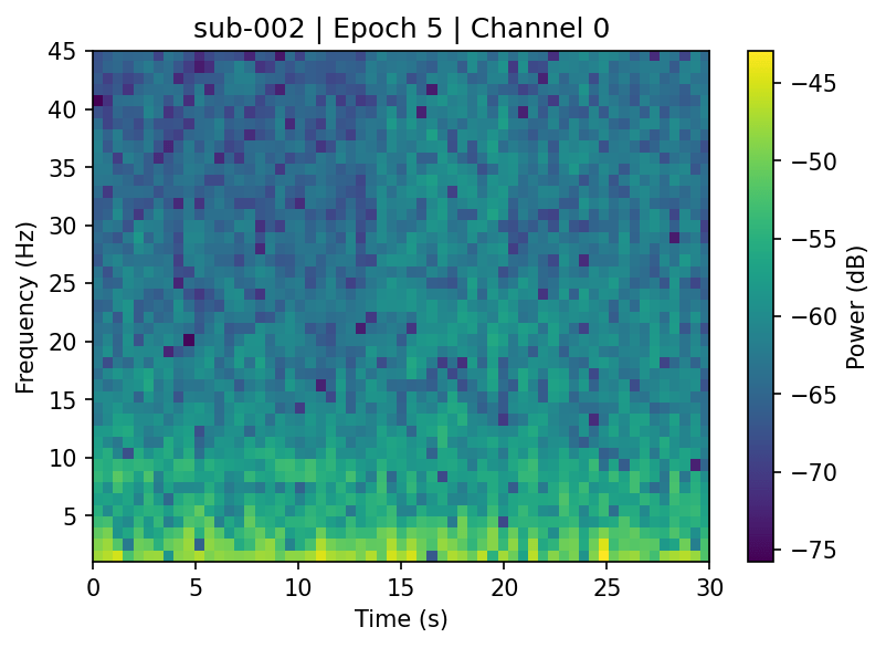
After computing the STFT spectrogram for each epoch, we restricted the frequency range from 0.5 to 45hz to focus on physiologically meaningful EEG activity. This band encompasses the canonical EEG frequency ranges (delta, theta, alpha, beta, and gamma) associated with cognitive and pathological processes, while attenuating slow baseline drifts below 0.5 Hz and high-frequency components dominated by line noise and electromyographic artifacts. Similar band-limiting strategies have been widely adopted in prior EEG studies to improve signal quality and analytical robustness. [39], [28]

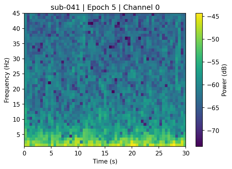
Fig. 2. Displayed are images of Alzheimer’s patient’s spectrograms (a) and healthy control (b) after applying a frequency mask between 0.5 and 45 Hz.

Data Normalization

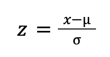
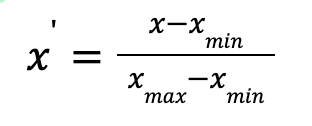
After extracting STFT spectrograms, two data transformation methods were evaluated: min-max normalization and z-score standardization. Min-max normalization scales the data output range from  $A_min$ to $A_max$while standardization transforms the data by centering it around the mean and scaling based on the standard deviation. Data transformation plays an important role in ensuring consistency and comparability of features. This step ensures that the model learns patterns relevant to the task, rather than being influenced by scale differences in the input data. In our approach, we applied scaling methods across epochs to ensure each epoch contributed equally to model training, preventing differences from different segments from dominating the learned representations and model outcome. [23], [40], [41], [42]. After testing both data transformation methods, z-score standardization had better accuracy against min-max normalization (90.75% vs. 87.91% accuracy, respectively).

Z-Score Standardization is calculated as: $z=(x-μ)/σ$

The Min-Max normalization is calculated as:

Classification

This section discusses the proposed CSA-net and the algorithms employed to optimally tune the model.

Model

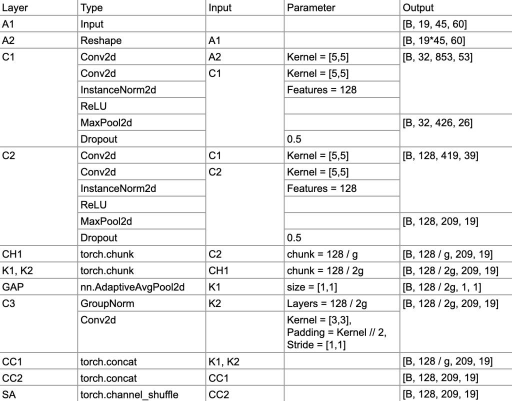
The CSA-net model first receives the input $Xᵢ∈R^((B ”x”  C × H × W) )$, where B denotes the batch size for the neural network, C denotes the number of channels, and H and W denote the height and width of the STFT spectrogram, respectively. To enable two-dimensional convolutional processing, the input tensor is reshaped along the channel dimension, thereby collapsing the height and channel dimensions, resulting in a tensor shape of $Xᵢ∈R^((B ” x ” (C ⋅ H) × W) ).$The reshaped tensor is used as the input for the convolutional block, which includes 2 two-dimension convolutional layers, instance normalization, Relu activation and dropout followed by a shuffle attention block. Finally, the output is flattened along the channel dimension, resulting in a tensor shape of $Xᵢ∈R^(B ” x ” (C ⋅ H ⋅ W)$ to be used in the feed-forward network (FFN) layer, which determines the class of the input. The detailed model architecture is summarized in Figure 3.

Early stoppage was performed to determine the best number of epochs (number of epochs represents the number of times data moves within the model in a forward and backward direction) [43]. The dataset was partitioned into training, validation, and test sets in a 70%, 15%, and 15% split, respectively, with model performance on the validation set evaluated after each epoch. Training was terminated when the validation loss failed to improve for three consecutive epochs, at which point the model parameters corresponding to the lowest validation loss were retained.

Convolutional block

Convolutional layers form the core computational mechanism of convolutional neural networks, enabling systematic feature extraction across images and matrices. Each convolution operation applies a learnable kernel to local regions of the input STFT spectrogram, computes element-wise products, and aggregates the results to produce an output value at the corresponding spatial location. Repeating this operation across the entire input yields a feature map that encodes localized spectro-temporal patterns relevant for downstream processing [44].

To capture local spectro-temporal patterns while preserving signal structure, two convolutional layers were employed with a kernel size of $5 × 5$, stride = 1, and padding = 1. This configuration enables the extraction of localized frequency-time relationships from the input matrix while ensuring that boundary regions are processed consistently with central regions. The use of kernels larger than a single time or frequency point allows the network to model interactions across neighboring frequency bands and adjacent time steps. Collectively, these convolutional operations reduce the effective dimensionality of the representation for subsequent layers while exposing salient spectro-temporal features.

Instance Normalization

EEG recordings exhibit significant variability across subjects due to differences in recording sessions and acquisition hardware. This variability introduces domain-specific shifts in signal distributions that can negatively impact the generalization performance of deep learning models [45]. Conventional normalization methods such as batch normalization or layer normalization can remove subject-specific or clinically relevant characteristics or introduce data leakage across patients, thereby reducing the discriminative power of the model [46]. To mitigate these effects, instance normalization was applied to preserve epoch-level feature structure while maintaining discriminative capacity across classes and subjects. [47], [48].

Shuffle Attention

Attention mechanisms, motivated by principles of the human visual system, enable neural networks to selectively emphasize informative components of the input while suppressing less relevant features [49]. This narrow focus and biasing of pertinent information facilitates the understanding of the model to create more accurate predictions. In natural language processing, attention allows models to weight words or phrases according to their contextual importance, whereas in image classification it highlights spatial regions or feature channels that contribute most strongly to the prediction [50].

Shuffle attention integrates two widely used attention paradigms in computer vision – channel attention and spatial attention – to enhance feature representations through complementary aggregation and transformation operations [51]. In this architecture, the input feature map is partitioned into subgroups, within which channel and spatial attention are jointly applied. The resulting features are then aggregated and concatenated, followed by a channel shuffle operation that promotes information exchange across feature groups.

Grouping

Given an input feature map $X ∈ R^(C ×H × W)$where $C, H, W$ denote the channel, height, and width, respectively, the shuffle attention module partitions X into G groups along the channel dimension, yielding sub-tensors $X =[ X_1, …, X_g ],$ $X_k ∈ R^(C/G ×H ×W).$ Each group $X_k$ is then evenly divided along the channel dimension into two subcomponents, generating $X_k1, X_k2 ∈ R^(C/2G × H × W).$This partitioning enables the parallel application of channel attention and spatial attention within each group, allowing the model to capture complementary information related to feature importance (“what”) and spatial relevance (“where”).

$X_k = [X_k1, X_k2 ], where X_k1, X_k2 ∈ R^(C/2G × H × W)$

Channel Attention

To capture channel-specific information, global average pooling is applied to compute channel-wise summary statistics, which are then passed through a fully connected layer to generate adaptive channel weights. A sigmoid activation maps these weights to the [0, 1] range, and the resulting coefficients are applied multiplicatively to the original feature map $X_k1$.

$V_k1= Sigmoid(FC(AvgPool(X_k1 )))$

$Z_k1= X_k1 ⊙ V_k1$

Spatial Attention

Spatial attention complements channel attention by emphasizing where informative regions are located within the feature map. Group normalization is first applied to  to generate spatial-wise statistics, followed by a convolutional layer with a 3 × 3 kernel to model local spatial dependencies. A sigmoid activation is then applied to generate spatial attention weights, which are multiplied element-wise with the original feature map $X_k2$.

$M_k2 = Sigmoid(Conv_(3×3) (GN(X_k2 )))$

$Z_k2 = X_k2 ⊙ M_k2$

Concatenation and Channel Shuffling

The outputs of the channel and spatial attention modules are concatenated to form a processed feature group $Z_k.$ All $Z_k$ groups are then concatenated along the channel dimension to reconstruct a feature map with the same dimensionality as the original input $X$. A final channel shuffle operation is applied to facilitate information exchange across groups.

$Z_k = [Z_k1, Z_k2 ]$

$Z_out = CS([Z_1, Z_(2,)… Z_G ])$

Unlike approaches that insert attention modules after each convolutional layer, the shuffle attention mechanism was applied only after the final convolutional block. Applying attention at every stage can increase computational and memory overhead while providing limited performance gains, particularly when early-layer features are noisy and weakly semantic. Restricting attention to higher-level feature maps allows the model to emphasize salient spectro-temporal patterns extracted by the convolutional layers, thereby enhancing discriminative representations with reduced complexity [52].

Feed Forward Layer

For classification, the flattened feature representation was passed to a fully connected layer followed by a sigmoid cross-entropy activation to produce binary class predictions. Batch size was set to 64, learning was 0.0004 and L2 regularization weight decay was set to 0.0001. Model optimization was performed using AdamW, in which weight decay is decoupled from the gradient-based parameter updates. This decoupling prevents interference with adaptive learning rates and provides more consistent regularization compared with standard Adam, supporting improved generalization. [53].

Results and Discussion

Experimental Setup

The time-frequency and signal processing steps, including, EEG cleaning, segmentation and feature extraction were implemented in Python 3.12 MNE library. The deep learning model used was trained and validated with PyTorch 2.4, and the evaluation functions were implemented using the Scikit-Learn library.

Results

Raw EEG recordings acquired in a routine clinical setting were denoised, segmented into overlapping epochs, and finally transformed into time-frequency representations using the short-time Fourier Transform for binary classification of Alzheimer’s Disease against healthy patients. The dataset was then partitioned at the subject level into training, validation, and test sets using a 70%, 15%, and 15% split, respectively, to prevent data leakage. Data leakage occurs when information from the same subject appears across multiple data splits, leading to inflated performance estimates. In EEG-based Alzheimer’s classification, random epoch-wise splitting introduces patient-level (subject-wise) leakage because epochs from the same individual are highly correlated. To mitigate this issue, all splits were performed at the patient level, ensuring that no epochs from a given subject were shared across training, validation, or testing sets [5]. Young et al. [54] found that data leakage is the most powerful and recurrent source of performance inflation in deep-learning (DL) studies of Alzheimer’s disease (AD). Deep learning models often claim high accuracy, exceeding 95%, yet fail in clinical translation because neural networks excel at detecting subtle patterns within features. When splitting the dataset by epoch from the same patient, the model is more likely to memorize patient-specific signatures rather than disease-related features. In essence, the model remembers patients rather than pathology, a form of overfitting that produces inflated results but has zero clinical utility. Yagis et al. [55] evaluated a model with the same dataset under two different validation methods: slice-wise splitting and patient-wise splitting, yielding 94% and 66% accuracy, respectively. This 28-percentage-point difference is attributed solely to the data split. These inflated performance metrics can cause serious clinical implications by creating unrealistic expectations among clinicians, patients, funding bodies and an erosion of trust in AI solutions following real-world failures. Healthcare systems may prematurely invest in AI tools to assist in diagnosis that ultimately fail when deployed on real-world data, while patients and families desperate for early diagnosis may be given false hope about the realistic capabilities of AI-assisted diagnosis. This ultimately undermines the trust and legitimacy of AI advancements and predictions and delays the implementation of these tools in a clinical setting.

Table 1: Model Evaluation Metrics

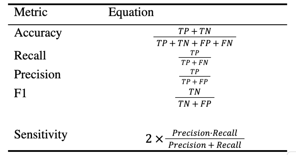
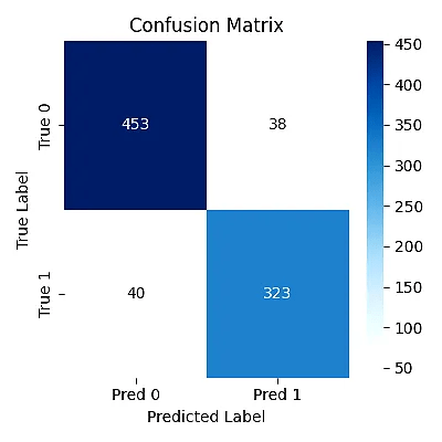
Using subject-wise validation, the proposed model achieved an accuracy, recall, precision, F1 score, and specificity of 90.87%, 89.47%, 88.98%, 89.23%, and 92.36%, respectively. A confusion matrix is a metric table used to display and evaluate the findings of a classification algorithm by calculating statistical measures [56]. Figure 4 displays a confusion matrix of how well our binary classification (AD vs HC) performed against actual labels, revealing True Positives (TP), True Negatives (TN), False Positives (FP) and False Negatives (FN) [57]. Although higher accuracies exceeding 95% have been reported in studies employing epoch-level splitting, such estimates are susceptible to subject-level data leakage. In contrast, the performance obtained here reflects a more conservative but clinically realistic evaluation of model generalization.

Table 2: Performance Comparison of Machine Learning Models

Model	Accuracy	Recall	Precision	F1	Sensitivity
PSA-Net	82.55%	65.29%	91.15%	76.08%	92.30%
CBAM	85.71%	88.71%	79.90%	84.07%	83.50%
Coordinate	87.47%	85.12%	85.36%	85.24%	89.20%
CNN + LSTM	84.06%	70.78%	89.58%	79.08%	93.9%
2d CNN	84.24%	80.25%	82.28%	81.25%	87.20%
CSA-NET	90.87%	89.47%	88.98%	89.23%	92.36%

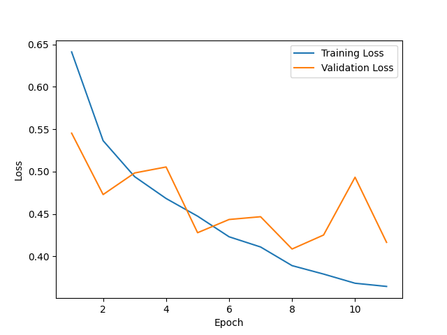
Early stopping was applied to mitigate overfitting and retain the model corresponding to the lowest validation loss. Validation loss was monitored after each epoch with a patience of three epochs. As shown in Figure 5, training loss decreased monotonically, indicating effective optimization of the model parameters. Validation loss initially decreased in parallel with training loss, suggesting adequate generalization; however, after 11 epochs, validation loss plateaued while training loss continued to decrease, indicating the onset of overfitting [58]. The limited number of training epochs is consistent with the modest dataset size and substantial inter-subject variability typical of biomedical EEG data.

To assess the effectiveness of the proposed approach, the model was compared with several established architectures and attention mechanisms, as summarized in Table 3. Shuffle attention was evaluated against CBAM (convolutional block attention mechanism) [10], CA (coordinate attention) [59], PSA-net (point-wise spatial attention network) [60], along with a convolutional neural network with a long-short-term-memory (CNN-LSTM) module [61] to account for sequential dependencies in STFT spectrograms. Hyperparameters, including learning rate, early stopping criteria, L2 weight decay, and dropout rate, were held constant across all experiments. In addition, an ablation experiment using a two-dimensional convolutional neural network without attention resulted in reduced performance, supporting the contribution of the shuffle attention module.

The leave-one-subject-out (LOSO) validation strategy was used to further evaluate the model’s ability to generalize to unseen individuals. Under this scheme, data from one subject were held out for testing while the remaining subjects’ data were used for training, and this process was repeated iteratively for each subject. Performance metrics were then aggregated across all folds, providing a direct assessment of subject-level generalization [62]. Using LOSO validation, the model achieved an accuracy of 81.43%, recall of 83.85%, precision of 81.21%, and F1 score of 84.71%. The performance gap observed between holdout validation and LOSO cross-validation reflects the substantial inter-subject variability inherent in EEG data and the associated challenge of robust subject-level discrimination.

Discussion

The proposed methodology integrates a shuffle attention mechanism at the output of the convolutional feature extractor to discriminate between Alzheimer’s disease (AD) and healthy control (HC) subjects. The workflow begins with raw EEG recordings acquired under routine clinical conditions, with no reported dementia-related comorbidities. Signals were denoised using Artifact Subspace Reconstruction and independent component analysis to remove non-neural artifacts. The cleaned recordings were segmented into 30s epochs with 50% overlap, after which short-time Fourier transform (STFT) spectrograms were computed and band-limited to 0.5-45 Hz to obtain time-frequency representations. A deep neural network comprising two convolutional layers, a shuffle attention module, and a fully connected classifier was then trained. Model performance was evaluated using both leave-one-subject-out (LOSO) cross-validation and a 70/15/15 subject-wise holdout split.

Prior studies have investigated EEG-based dementia detection using a range of machine learning approaches [63]. The most advanced and recent studies usually propose a deep neural network architecture that first processes the time-domain signal through a time-frequency transform such as a Wavelet Transform [64] or Continuous Wavelet Transform [65] and then utilizes the capabilities of a Convolutional layer to extract salient features or neural networks such as autoencoders to efficiently learn data representations while down-sampling [66]. Although attention mechanisms have been incorporated in some studies to enhance feature discrimination [65], [67], many rely on epoch-wise or slice-wise data partitioning, which introduces subject-level data leakage and limits clinical interpretability. To the best of our knowledge, this study is the first to combine a shuffle attention mechanism with a convolutional neural network under a strictly enforced subject-wise validation protocol. By emphasizing salient time-frequency features while suppressing subject-specific noise patterns, the proposed approach jointly addresses feature selection and validation rigor, contributing to improved robustness and potential clinical relevance. Although some studies report classification accuracies exceeding 95%, such performance is typically obtained using epoch-wise or slice-wise data splitting and is therefore susceptible to subject-level data leakage. In contrast, the more conservative performance observed here better reflects real-world clinical conditions, in which models are evaluated on previously unseen patients. The performance reduction observed under LOSO cross-validation highlights the substantial inter-subject variability inherent in EEG data and reinforces the necessity of subject-wise validation in neuropsychological deep learning studies.

Limitations

Several limitations should be acknowledged. First, although the dataset is sufficient for methodological evaluation, its size limits the model’s ability to generalize broadly. Validation on larger and more diverse cohorts is required to establish robustness across populations. Second, the proposed convolutional architecture depends on a fixed electrode configuration. EEG recordings are acquired using predefined montages, and the learned convolutional kernels implicitly assume a consistent channel arrangement and input dimensionality. Consequently, models trained on a specific electrode setup may not generalize to datasets acquired with different electrode configurations, restricting applicability across heterogeneous EEG systems.

An additional limitation concerns the choice of window segmentation (30s 21 with 50% overlap), which differs from the shorter epoch durations (typically < 5 s) commonly used in EEG-based machine learning studies [68], [69]. Shorter windows are often adopted due to the classifier’s inability to capture long-range dependencies and the size of the dataset, which necessitates the need to generate a lot of training samples from a small duration of EEG recordings. In the present study, longer temporal context was accommodated through the use of 5 × 5 convolutional kernels and multiple convolutional layers, which expand the receptive field and enable the extraction of longer-range spectro-temporal features.

Finally, although this work emphasizes algorithmic development, clinical applicability requires validation on larger datasets collected across multiple medical centers. Future studies should include more diverse patient populations and additional diagnostic categories, such as mild cognitive impairment and other neurological conditions, to better reflect real-world clinical scenarios. Addressing these limitations is essential for improving cross-dataset robustness and advancing the deployment of EEG-based deep learning models in clinical practice.

Conclusion

This study evaluated the effectiveness of integrating a shuffle attention mechanism into a convolutional deep learning architecture for binary classification of Alzheimer’s disease versus healthy controls. Model performance was assessed using a clinical EEG dataset acquired at AHEPA General Hospital of Thessaloniki, Greece, under a strictly enforced subject-wise validation protocol. The proposed approach achieved an accuracy of 90.87%, recall of 89.47%, precision of 88.98%, F1 score of 89.23%, and specificity of 92.36%, indicating effective extraction of discriminative time-frequency features from EEG signals. These results contribute to the growing literature on EEG-based Alzheimer’s disease classification using machine learning methods and highlight the importance of combining attention mechanisms with rigorous validation strategies.

Acknowledgements. This work was supported by Open Labs, an open-source pedagogical framework and continuous-feedback software designed to foster a community of creative thinkers and researchers. We would like to express our eternal gratitude to Decoded Brain, an active student-led research organization of scientists and engineers whose ecosystem and creation of Open Labs made the development and execution of this research possible.

Disclosures. The authors declare no conflicts of interest.